Ykhjuy

In mathematics, a linear map (also called a linear mapping, linear transformation or, in some contexts, linear function) is a mapping V → W between two modules (including vector spaces) that preserves (in the sense defined below) the operations of addition and scalar multiplication.

An important special case is when V = W, in which case the map is called a linear operator,^[1] or an endomorphism of V. Sometimes the term linear function has the same meaning as linear map, while in analytic geometry it does not.

A linear map always maps linear subspaces onto linear subspaces (possibly of a lower dimension);^[2] for instance it maps a plane through the origin to a plane, straight line or point. Linear maps can often be represented as matrices, and simple examples include rotation and reflection linear transformations.

In the language of abstract algebra, a linear map is a module homomorphism. In the language of category theory it is a morphism in the category of modules over a given ring.

Definition and first consequences

Let V{textstyle V} and W{textstyle W} be vector spaces over the same field K.{textstyle mathbf {K} .} A function f:V→W{textstyle f:Vto W} is said to be a linear map if for any two vectors u,v∈V{textstyle mathbf {u} ,mathbf {v} in V} and any scalar c∈K{textstyle cin mathbf {K} } the following two conditions are satisfied:

f(u+v)=f(u)+f(v){displaystyle f(mathbf {u} +mathbf {v} )=f(mathbf {u} )+f(mathbf {v} )}	additivity / operation of addition
f(cu)=cf(u){displaystyle f(cmathbf {u} )=cf(mathbf {u} )}	homogeneity of degree 1 / operation of scalar multiplication

Thus, a linear map is said to be operation preserving. In other words, it does not matter whether you apply the linear map before or after the operations of addition and scalar multiplication.

This is equivalent to requiring the same for any linear combination of vectors, i.e. that for any vectors u1,…,un∈V{textstyle mathbf {u} _{1},ldots ,mathbf {u} _{n}in V} and scalars c1,…,cn∈K,{textstyle c_{1},ldots ,c_{n}in mathbf {K} ,} the following equality holds:^[3][4]

f(c1u1+⋯+cnun)=c1f(u1)+⋯+cnf(un).{displaystyle fleft(c_{1}mathbf {u} _{1}+cdots +c_{n}mathbf {u} _{n}right)=c_{1}fleft(mathbf {u} _{1}right)+cdots +c_{n}fleft(mathbf {u} _{n}right).}

Denoting the zero elements of the vector spaces V{textstyle V} and W{textstyle W} by 0V{textstyle mathbf {0} _{V}} and 0W{textstyle mathbf {0} _{W}} respectively, it follows that f(0V)=0W.{textstyle fleft(mathbf {0} _{V}right)=mathbf {0} _{W}.} Let c=0{textstyle c=0} and v∈V{textstyle mathbf {v} in V} in the equation for homogeneity of degree 1:

f(0V)=f(0v)=0f(v)=0W.{displaystyle fleft(mathbf {0} _{V}right)=fleft(0mathbf {v} right)=0f(mathbf {v} )=mathbf {0} _{W}.}

Occasionally, V{textstyle V} and W{textstyle W} can be considered to be vector spaces over different fields. It is then necessary to specify which of these ground fields is being used in the definition of "linear". If V{textstyle V} and W{textstyle W} are considered as spaces over the field K{textstyle mathbf {K} } as above, we talk about K{textstyle mathbf {K} }-linear maps. For example, the conjugation of complex numbers is an R{textstyle mathbf {R} }-linear map C→C{textstyle mathbf {C} to mathbf {C} }, but it is not C{textstyle mathbf {C} }-linear.

A linear map V→K{textstyle Vto mathbf {K} } with K{textstyle mathbf {K} } viewed as a vector space over itself is called a linear functional.^[5]

These statements generalize to any left-module RM{textstyle {}_{R}M} over a ring R{textstyle R} without modification, and to any right-module upon reversing of the scalar multiplication.

Examples

• The zero map x ↦ 0 between two left-modules (or two right-modules) over the same ring is always linear.


• The identity map on any module is a linear operator.


• Any homothecy centered in the origin of a vector space, v↦cv{textstyle vmapsto cv} where c is a scalar, is a linear operator. This does not hold in general for modules, where such a map might only be semilinear.


• For real numbers, the map x ↦ x² is not linear.


• For real numbers, the map x ↦ x + 1 is not linear (but is an affine transformation; y = x + 1 is a linear equation, as the term is used in analytic geometry.)


• If A is a real m × n matrix, then A defines a linear map from Rⁿ to R^m by sending the column vector x ∈ Rⁿ to the column vector Ax ∈ R^m. Conversely, any linear map between finite-dimensional vector spaces can be represented in this manner; see the following section.


• 
  Differentiation defines a linear map from the space of all differentiable functions to the space of all functions. It also defines a linear operator on the space of all smooth functions.


• The (definite) integral over some interval I is a linear map from the space of all real-valued integrable functions on I to R.


• The (indefinite) integral (or antiderivative) with a fixed starting point defines a linear map from the space of all real-valued integrable functions on R to the space of all real-valued, differentiable, functions on R. Without a fixed starting point, an exercise in group theory will show that the antiderivative maps to the quotient space of the differentiables over the equivalence relation, "differ by a constant", which yields an identity class of the constant valued functions (∫: I(ℜ) → D(ℜ)/ℜ){textstyle left(,int !: I(Re ) to D(Re )/Re ,right)}.


• If V and W are finite-dimensional vector spaces over a field F, then functions that send linear maps f : V → W to dim_F(W) × dim_F(V) matrices in the way described in the sequel are themselves linear maps (indeed linear isomorphisms).


• The expected value of a random variable (which is in fact a function, and as such a member of a vector space) is linear, as for random variables X and Y we have E[X + Y] = E[X] + E[Y] and E[aX] = aE[X], but the variance of a random variable is not linear.

• 
  

  

  
  

  
  

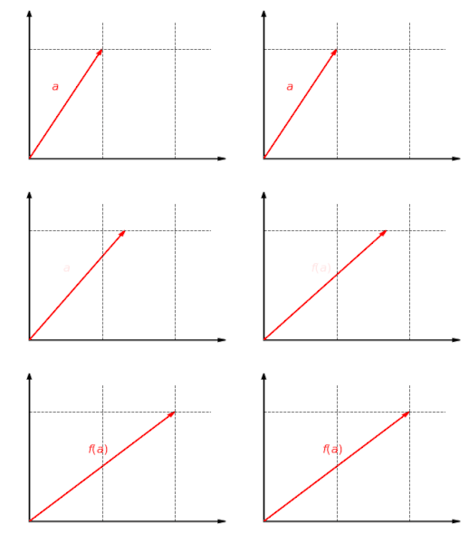
  The function f:R2→R2{textstyle f:mathbb {R} ^{2}to mathbb {R} ^{2}} with f(x,y)=(2x,y){textstyle f(x,y)=(2x,y)} is a linear map. This function scales the x{textstyle x} component of a vector by the factor 2{textstyle 2}.
  

  
  

  
  


• 
  

  

  
  

  
  

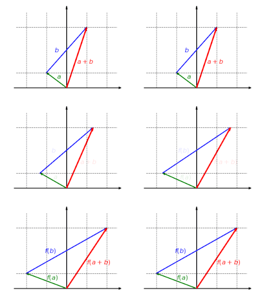
  The function is additive: It doesn't matter whether first vectors are added and then mapped or whether they are mapped and finally added: f(a+b)=f(a)+f(b){textstyle f(a+b)=f(a)+f(b)}
  

  
  

  
  


• 
  

  

  
  

  
  

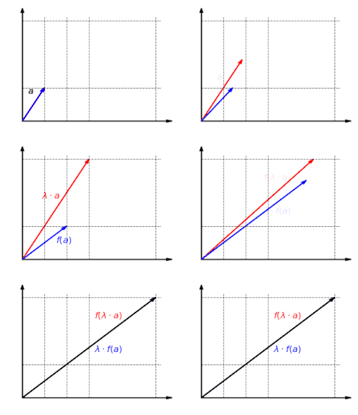
  The function is homogeneous: It doesn't matter whether a vector is first scaled and then mapped or first mapped and then scaled: f(λa)=λf(a){textstyle f(lambda a)=lambda f(a)}
  

  
  

  
  

Matrices

If V and W are finite-dimensional vector spaces and a basis is defined for each vector space, then every linear map from V to W can be represented by a matrix.^[6] This is useful because it allows concrete calculations. Matrices yield examples of linear maps: if A is a real m × n matrix, then f(x) = Ax describes a linear map Rⁿ → R^m (see Euclidean space).

Let {v₁, …, v_n} be a basis for V. Then every vector v in V is uniquely determined by the coefficients c₁, …, c_n in the field R:

c1v1+⋯+cnvn.{displaystyle c_{1}mathbf {v} _{1}+cdots +c_{n}mathbf {v} _{n}.}

If f : V → W is a linear map,

f(c1v1+⋯+cnvn)=c1f(v1)+⋯+cnf(vn),{displaystyle fleft(c_{1}mathbf {v} _{1}+cdots +c_{n}mathbf {v} _{n}right)=c_{1}fleft(mathbf {v} _{1}right)+cdots +c_{n}fleft(mathbf {v} _{n}right),}

which implies that the function f is entirely determined by the vectors f(v₁), …, f(v_n). Now let {w₁, …, w_m} be a basis for W. Then we can represent each vector f(v_j) as

f(vj)=a1jw1+⋯+amjwm.{displaystyle fleft(mathbf {v} _{j}right)=a_{1j}mathbf {w} _{1}+cdots +a_{mj}mathbf {w} _{m}.}

Thus, the function f is entirely determined by the values of a_ij. If we put these values into an m × n matrix M, then we can conveniently use it to compute the vector output of f for any vector in V. To get M, every column j of M is a vector

(a1j⋯amj)T{displaystyle {begin{pmatrix}a_{1j}&cdots &a_{mj}end{pmatrix}}^{textsf {T}}}

corresponding to f(v_j) as defined above. To define it more clearly, for some column j that corresponds to the mapping f(v_j),

M=( ⋯a1j⋯ ⋮amj){displaystyle mathbf {M} ={begin{pmatrix} cdots &a_{1j}&cdots \&vdots &\&a_{mj}&end{pmatrix}}}

where M is the matrix of f. In other words, every column j = 1, …, n has a corresponding vector f(v_j) whose coordinates a_1j, …, a_mj are the elements of column j. A single linear map may be represented by many matrices. This is because the values of the elements of a matrix depend on the bases chosen.

The matrices of a linear transformation can be represented visually:

1. Matrix for T{textstyle T} relative to B{textstyle B}: A{textstyle A}
   


2. Matrix for T{textstyle T} relative to B′{textstyle B'}: A′{textstyle A'}
   


3. Transition matrix from B′{textstyle B'} to B{textstyle B}: P{textstyle P}
   


4. Transition matrix from B{textstyle B} to B′{textstyle B'}: P−1{textstyle P^{-1}}
   

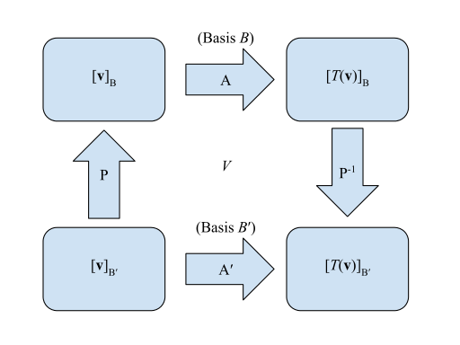
Such that starting in the bottom left corner [v→]B′{textstyle left[{vec {v}}right]_{B'}} and looking for the bottom right corner [T(v→)]B′{textstyle left[Tleft({vec {v}}right)right]_{B'}}, one would left-multiply—that is, A′[v→]B′=[T(v→)]B′{textstyle A'left[{vec {v}}right]_{B'}=left[Tleft({vec {v}}right)right]_{B'}}. The equivalent method would be the "longer" method going clockwise from the same point such that [v→]B′{textstyle left[{vec {v}}right]_{B'}} is left-multiplied with P−1AP{textstyle P^{-1}AP}, or P−1AP[v→]B′=[T(v→)]B′{textstyle P^{-1}APleft[{vec {v}}right]_{B'}=left[Tleft({vec {v}}right)right]_{B'}}.

Examples of linear transformation matrices

In two-dimensional space R² linear maps are described by 2 × 2 real matrices. These are some examples:

• 
  rotation
  
  
  
  • by 90 degrees counterclockwise:
    

    A=(0−110){displaystyle mathbf {A} ={begin{pmatrix}0&-1\1&0end{pmatrix}}}

    
    
  
  
  • by an angle θ counterclockwise:
    

    A=(cos⁡θ−sin⁡θsin⁡θcos⁡θ){displaystyle mathbf {A} ={begin{pmatrix}cos theta &-sin theta \sin theta &cos theta end{pmatrix}}}

    
    
  
  
  
  


• 
  reflection
  
  
  
  • about the x axis:
    

    A=(100−1){displaystyle mathbf {A} ={begin{pmatrix}1&0\0&-1end{pmatrix}}}

    
    
  
  
  • about the y axis:
    

    A=(−1001){displaystyle mathbf {A} ={begin{pmatrix}-1&0\0&1end{pmatrix}}}

    
    
  
  
  
  


• 
  scaling by 2 in all directions:
  

  A=(2002)=2I{displaystyle mathbf {A} ={begin{pmatrix}2&0\0&2end{pmatrix}}=2mathbf {I} }

  
  


• 
  horizontal shear mapping:
  

  A=(1m01){displaystyle mathbf {A} ={begin{pmatrix}1&m\0&1end{pmatrix}}}

  
  


• 
  squeeze mapping:
  

  A=(k001k){displaystyle mathbf {A} ={begin{pmatrix}k&0\0&{frac {1}{k}}end{pmatrix}}}

  
  


• 
  projection onto the y axis:
  

  A=(0001).{displaystyle mathbf {A} ={begin{pmatrix}0&0\0&1end{pmatrix}}.}

  
  

Forming new linear maps from given ones

The composition of linear maps is linear: if f : V → W and g : W → Z are linear, then so is their composition g ∘ f : V → Z. It follows from this that the class of all vector spaces over a given field K, together with K-linear maps as morphisms, forms a category.

The inverse of a linear map, when defined, is again a linear map.

If f₁ : V → W and f₂ : V → W are linear, then so is their pointwise sum f₁ + f₂ (which is defined by (f₁ + f₂)(x) = f₁(x) + f₂(x)).

If f : V → W is linear and a is an element of the ground field K, then the map af, defined by (af)(x) = a(f(x)), is also linear.

Thus the set L(V, W) of linear maps from V to W itself forms a vector space over K, sometimes denoted Hom(V, W). Furthermore, in the case that V = W, this vector space (denoted End(V)) is an associative algebra under composition of maps, since the composition of two linear maps is again a linear map, and the composition of maps is always associative. This case is discussed in more detail below.

Given again the finite-dimensional case, if bases have been chosen, then the composition of linear maps corresponds to the matrix multiplication, the addition of linear maps corresponds to the matrix addition, and the multiplication of linear maps with scalars corresponds to the multiplication of matrices with scalars.

Endomorphisms and automorphisms

A linear transformation f: V → V is an endomorphism of V; the set of all such endomorphisms End(V) together with addition, composition and scalar multiplication as defined above forms an associative algebra with identity element over the field K (and in particular a ring). The multiplicative identity element of this algebra is the identity map id: V → V.

An endomorphism of V that is also an isomorphism is called an automorphism of V. The composition of two automorphisms is again an automorphism, and the set of all automorphisms of V forms a group, the automorphism group of V which is denoted by Aut(V) or GL(V). Since the automorphisms are precisely those endomorphisms which possess inverses under composition, Aut(V) is the group of units in the ring End(V).

If V has finite dimension n, then End(V) is isomorphic to the associative algebra of all n × n matrices with entries in K. The automorphism group of V is isomorphic to the general linear group GL(n, K) of all n × n invertible matrices with entries in K.

Kernel, image and the rank–nullity theorem

If f : V → W is linear, we define the kernel and the image or range of f by

ker⁡(f)={x∈V:f(x)=0}im⁡(f)={w∈W:w=f(x),x∈V}{displaystyle {begin{aligned}operatorname {ker } (f)&={,xin V:f(x)=0,}\operatorname {im} (f)&={,win W:w=f(x),xin V,}end{aligned}}}

ker(f) is a subspace of V and im(f) is a subspace of W. The following dimension formula is known as the rank–nullity theorem:

dim⁡(ker⁡(f))+dim⁡(im⁡(f))=dim⁡(V).{displaystyle dim(ker(f))+dim(operatorname {im} (f))=dim(V).}^[7]

The number dim(im(f)) is also called the rank of f and written as rank(f), or sometimes, ρ(f); the number dim(ker(f)) is called the nullity of f and written as null(f) or ν(f). If V and W are finite-dimensional, bases have been chosen and f is represented by the matrix A, then the rank and nullity of f are equal to the rank and nullity of the matrix A, respectively.

Cokernel

A subtler invariant of a linear transformation f:V→W{textstyle f:Vto W} is the cokernel, which is defined as

coker⁡(f):=W/f(V)=W/im⁡(f).{displaystyle operatorname {coker} (f):=W/f(V)=W/operatorname {im} (f).}

This is the dual notion to the kernel: just as the kernel is a subspace of the domain, the co-kernel is a quotient space of the target.
Formally, one has the exact sequence

0→ker⁡(f)→V→W→coker⁡(f)→0.{displaystyle 0to ker(f)to Vto Wto operatorname {coker} (f)to 0.}

These can be interpreted thus: given a linear equation f(v) = w to solve,

• the kernel is the space of solutions to the homogeneous equation f(v) = 0, and its dimension is the number of degrees of freedom in a solution, if it exists;


• the co-kernel is the space of constraints that must be satisfied if the equation is to have a solution, and its dimension is the number of constraints that must be satisfied for the equation to have a solution.

The dimension of the co-kernel and the dimension of the image (the rank) add up to the dimension of the target space. For finite dimensions, this means that the dimension of the quotient space W/f(V) is the dimension of the target space minus the dimension of the image.

As a simple example, consider the map f: R² → R², given by f(x, y) = (0, y). Then for an equation f(x, y) = (a, b) to have a solution, we must have a = 0 (one constraint), and in that case the solution space is (x, b) or equivalently stated, (0, b) + (x, 0), (one degree of freedom). The kernel may be expressed as the subspace (x, 0) < V: the value of x is the freedom in a solution – while the cokernel may be expressed via the map W → R, (a,b)↦(a):{textstyle (a,b)mapsto (a):} given a vector (a, b), the value of a is the obstruction to there being a solution.

An example illustrating the infinite-dimensional case is afforded by the map f: R^∞ → R^∞, {an}↦{bn}{textstyle left{a_{n}right}mapsto left{b_{n}right}} with b₁ = 0 and b_{n + 1} = a_n for n > 0. Its image consists of all sequences with first element 0, and thus its cokernel consists of the classes of sequences with identical first element. Thus, whereas its kernel has dimension 0 (it maps only the zero sequence to the zero sequence), its co-kernel has dimension 1. Since the domain and the target space are the same, the rank and the dimension of the kernel add up to the same sum as the rank and the dimension of the co-kernel ( ℵ0+0=ℵ0+1{textstyle aleph _{0}+0=aleph _{0}+1} ), but in the infinite-dimensional case it cannot be inferred that the kernel and the co-kernel of an endomorphism have the same dimension (0 ≠ 1). The reverse situation obtains for the map h: R^∞ → R^∞, {an}↦{cn}{textstyle left{a_{n}right}mapsto left{c_{n}right}} with c_n = a_{n + 1}. Its image is the entire target space, and hence its co-kernel has dimension 0, but since it maps all sequences in which only the first element is non-zero to the zero sequence, its kernel has dimension 1.

Index

For a linear operator with finite-dimensional kernel and co-kernel, one may define index as:

ind⁡(f):=dim⁡(ker⁡(f))−dim⁡(coker⁡(f)),{displaystyle operatorname {ind} (f):=dim(ker(f))-dim(operatorname {coker} (f)),}

namely the degrees of freedom minus the number of constraints.

For a transformation between finite-dimensional vector spaces, this is just the difference dim(V) − dim(W), by rank–nullity. This gives an indication of how many solutions or how many constraints one has: if mapping from a larger space to a smaller one, the map may be onto, and thus will have degrees of freedom even without constraints. Conversely, if mapping from a smaller space to a larger one, the map cannot be onto, and thus one will have constraints even without degrees of freedom.

The index of an operator is precisely the Euler characteristic of the 2-term complex 0 → V → W → 0. In operator theory, the index of Fredholm operators is an object of study, with a major result being the Atiyah–Singer index theorem.^[8]

Algebraic classifications of linear transformations

No classification of linear maps could hope to be exhaustive. The following incomplete list enumerates some important classifications that do not require any additional structure on the vector space.

Let V and W denote vector spaces over a field, F. Let T: V → W be a linear map.

• 
  T is said to be injective or a monomorphism if any of the following equivalent conditions are true:
  
  
  
  • 
    T is one-to-one as a map of sets.
  
  
  • kerT = {0_V}
  
  
  • 
    T is monic or left-cancellable, which is to say, for any vector space U and any pair of linear maps R: U → V and S: U → V, the equation TR = TS implies R = S.
  
  
  • 
    T is left-invertible, which is to say there exists a linear map S: W → V such that ST is the identity map on V.
  
  
  
  


• 
  T is said to be surjective or an epimorphism if any of the following equivalent conditions are true:
  
  
  
  • 
    T is onto as a map of sets.
  
  
  • 
    coker T = {0_W}
  
  
  • 
    T is epic or right-cancellable, which is to say, for any vector space U and any pair of linear maps R: W → U and S: W → U, the equation RT = ST implies R = S.
  
  
  • 
    T is right-invertible, which is to say there exists a linear map S: W → V such that TS is the identity map on W.
  
  
  
  


• 
  T is said to be an isomorphism if it is both left- and right-invertible. This is equivalent to T being both one-to-one and onto (a bijection of sets) or also to T being both epic and monic, and so being a bimorphism.


• If T: V → V is an endomorphism, then:
  
  
  
  • If, for some positive integer n, the n-th iterate of T, Tⁿ, is identically zero, then T is said to be nilpotent.
  
  
  • If T² = T, then T is said to be idempotent
    
  
  
  • If T = kI, where k is some scalar, then T is said to be a scaling transformation or scalar multiplication map; see scalar matrix.
  
  
  
  

Change of basis

Given a linear map which is an endomorphism whose matrix is A, in the basis B of the space it transforms vector coordinates [u] as [v] = A[u]. As vectors change with the inverse of B (vectors are contravariant) its inverse transformation is [v] = B[v'].

Substituting this in the first expression

B[v′]=AB[u′]{displaystyle Bleft[v'right]=ABleft[u'right]}

hence

[v′]=B−1AB[u′]=A′[u′].{displaystyle left[v'right]=B^{-1}ABleft[u'right]=A'left[u'right].}

Therefore, the matrix in the new basis is A′ = B⁻¹AB, being B the matrix of the given basis.

Therefore, linear maps are said to be 1-co- 1-contra-variant objects, or type (1, 1) tensors.

Continuity

A linear transformation between topological vector spaces, for example normed spaces, may be continuous. If its domain and codomain are the same, it will then be a continuous linear operator. A linear operator on a normed linear space is continuous if and only if it is bounded, for example, when the domain is finite-dimensional.^[9] An infinite-dimensional domain may have discontinuous linear operators.

An example of an unbounded, hence discontinuous, linear transformation is differentiation on the space of smooth functions equipped with the supremum norm (a function with small values can have a derivative with large values, while the derivative of 0 is 0). For a specific example, sin(nx)/n converges to 0, but its derivative cos(nx) does not, so differentiation is not continuous at 0 (and by a variation of this argument, it is not continuous anywhere).

Applications

A specific application of linear maps is for geometric transformations, such as those performed in computer graphics, where the translation, rotation and scaling of 2D or 3D objects is performed by the use of a transformation matrix. Linear mappings also are used as a mechanism for describing change: for example in calculus correspond to derivatives; or in relativity, used as a device to keep track of the local transformations of reference frames.

Another application of these transformations is in compiler optimizations of nested-loop code, and in parallelizing compiler techniques.

See also

Wikibooks has a book on the topic of: Linear Algebra/Linear Transformations

• Affine transformation


• Linear equation


• Bounded operator


• Antilinear map


• Semilinear map


• Continuous linear operator


• Bent function

Notes

References

• 
  Halmos, Paul R. (1974). Finite-Dimensional Vector Spaces. New York: Springer-Verlag. ISBN 0-387-90093-4.
  


• 
  Horn, Roger A.; Johnson, Charles R. (2013). Matrix Analysis (Second ed.). Cambridge University Press. ISBN 978-0-521-83940-2.
  


• 
  Lang, Serge (1987), Linear Algebra (Third ed.), New York: Springer-Verlag, ISBN 0-387-96412-6
  


• 
  Rudin, Walter (1976). Principles of Mathematical Analysis (Third ed.). McGraw-Hill. ISBN 0-07-085613-3.
  


• 
  Rudin, Walter (1991). Functional Analysis (Second ed.). McGraw-Hill. ISBN 0-07-054236-8.